Kaplan-Meier Guideline Suggestions

Introduction

In this example, two key survival endpoints are analysed:

Progression-Free Survival (PFS): Defined as the time from treatment initiation to either disease progression or death.
Overall Survival (OS): Defined as the time from treatment initiation to death from any cause.

This vignette covers the following steps:

Preparation of the dataset.
Creation of time-to-event and event indicator variables.
Compute Kaplan-meier estimator and fitting of Kaplan-Meier curves
Visualization of survival curves accompanied by risk tables.

The approach presented here follows the recommendations provided by Daniel Sjoberg’s ggsurvfit package for generating publication-ready Kaplan-Meier plots.

First, install packages if needed and load them.

## Load libraries

library(grstat)
library(dplyr)
library(survival)
library(ggsurvfit)
library(glue)

Data Overview

The dataset used is an extension of the dataset provided by the ggsurvfit package. Additional variables were simulated to resemble to a typical dataset from an oncology clinical study, including information on progression status, survival times, and treatment characteristics. Note: In this example, the end date is determined using the pmax() function, which selects the latest available date from the following: date of death, last visit, last RECIST scan, last patient contact, end of treatment, or last follow-up.

## Display dataset

head(data_surv)
#> # A tibble: 6 × 6
#>      id death date_start date_progression date_end   surg                       
#>   <dbl> <dbl> <date>     <date>           <date>     <fct>                      
#> 1     1     1 2021-04-16 2021-04-18       2021-04-19 Limited Time Since Surgery 
#> 2     2     0 2021-05-20 2021-05-25       2021-05-28 Limited Time Since Surgery 
#> 3     3     1 2021-03-27 NA               2021-03-28 Limited Time Since Surgery 
#> 4     4     1 2021-05-14 NA               2021-05-15 Extended Time Since Surgery
#> 5     5     1 2021-05-27 NA               2021-05-28 Extended Time Since Surgery
#> 6     6     1 2021-06-06 NA               2021-06-09 Limited Time Since Surgery

dim(data_surv)
#> [1] 929   6

Data Preparation

Variable Creation

The purpose of this section is to create status and time variables for Progression-Free Survival (PFS) and Overall Survival (OS).

First, the variables time and status (indicating whether an event occurred or was censored) need to be created to enable the use of various functions.

Time variable: The time variable represents the duration from a defined starting point (e.g., diagnosis, study enrollment, or start of treatment) to the time at which the patient’s status is recorded (e.g. death, disease progression, recurrence or last news). It is a numeric variable measured in units such as days, months, or years, depending on the study’s duration and requirements.
Status variable: The status variable is binary, indicating whether the event has occurred (event = 1) or not (censored = 0) for each subject by the end of the study period.

An event (1) indicates that the subject experienced the event of interest (e.g., death, relapse, transplant failure, etc.).

Censored (0) refers to those subjects who did not experience the event during the study. For these individuals, the ‘time-to-event’ is considered censored, indicating that we only know they did not experience the event up to a certain point.

## Example

data_surv_v2 = data_surv %>%
  mutate(
    status_PFS = ifelse(!is.na(date_progression), 1, 0 ),
    date_status_pfs = pmin(date_progression,date_end, na.rm = TRUE),
    status_OS = death,
    date_status_OS = date_end,
    time_pfs = as.numeric(date_status_pfs-date_start)/30.5,
    time_OS = as.numeric(date_status_OS-date_start)/30.5
  ) %>% 
  select(id,time_pfs,time_OS,status_PFS,status_OS,surg)

head(data_surv_v2)
#> # A tibble: 6 × 6
#>      id time_pfs time_OS status_PFS status_OS surg                       
#>   <dbl>    <dbl>   <dbl>      <dbl>     <dbl> <fct>                      
#> 1     1   0.0611  0.0869          1         1 Limited Time Since Surgery 
#> 2     2   0.175   0.277           1         0 Limited Time Since Surgery 
#> 3     3   0.0487  0.0487          0         1 Limited Time Since Surgery 
#> 4     4   0.0220  0.0220          0         1 Extended Time Since Surgery
#> 5     5   0.0469  0.0469          0         1 Extended Time Since Surgery
#> 6     6   0.0811  0.0811          0         1 Limited Time Since Surgery

Kaplan-Meier Analysis

Generate survival estimates using `survfit2()`

We recommend using the ggsurvfit package which uses survfit2()with the following syntax:

km.model_PFS = survfit2(Surv(time_pfs, status_PFS) ~ surg, data = data_surv_v2)
km.model_PFS
#> Call: survfit(formula = Surv(time_pfs, status_PFS) ~ surg, data = data_surv_v2)
#> 
#>                                    n events median 0.95LCL 0.95UCL
#> surg=Limited Time Since Surgery  682    372  0.149   0.141   0.157
#> surg=Extended Time Since Surgery 247    111  0.149   0.141   0.197

# Specific time points can be chosen to extract the estimated survival probabilities and related statistics from the Kaplan-Meier survival model (km.model_PFS). Here, the time points were set at 0.05, 0.10, and 0.20.

tidy_survfit(km.model_PFS, times = c(0.05, 0.10, 0.20)) %>% 
  select(strata, time, n.risk, n.event, estimate, conf.high, conf.low)
#> # A tibble: 6 × 7
#>   strata                       time n.risk n.event estimate conf.high conf.low
#>   <fct>                       <dbl>  <dbl>   <dbl>    <dbl>     <dbl>    <dbl>
#> 1 Extended Time Since Surgery  0.05    136      60    0.723     0.786    0.665
#> 2 Extended Time Since Surgery  0.1     114       9    0.673     0.741    0.612
#> 3 Extended Time Since Surgery  0.2      39      41    0.403     0.486    0.333
#> 4 Limited Time Since Surgery   0.05    429     156    0.753     0.788    0.720
#> 5 Limited Time Since Surgery   0.1     368      32    0.695     0.733    0.659
#> 6 Limited Time Since Surgery   0.2     101     176    0.337     0.382    0.298

Generate survival curves

For full documentation on ggsurvfit, visit the ggsurvfit website.

To cite their work, refer to the following:

Sjoberg D, Baillie M, Fruechtenicht C, Haesendonckx S, Treis T (2025). ggsurvfit: Flexible Time-to-Event Figures.
R package version 1.1.0. Available at: https://www.danieldsjoberg.com/ggsurvfit/.

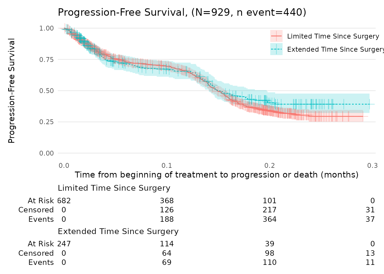
Progression-Free Survival (PFS)

km_PFS = survfit2(Surv(time_pfs, status_PFS) ~ surg, data = data_surv_v2) %>%
  ggsurvfit(linetype_aes = TRUE) +
  add_confidence_interval() +
  add_risktable(
    risktable_stats = c("n.risk", "cum.censor", "cum.event" )
  ) +
  theme_ggsurvfit_KMunicate() +
  scale_y_continuous(limits = c(0, 1)) +
  scale_x_continuous(expand = c(0.02, 0)) +
  theme(legend.position="inside", legend.position.inside = c(0.85, 0.85))
km_PFS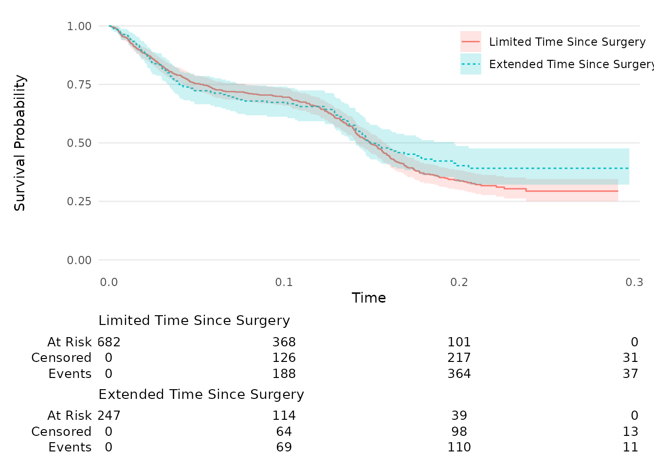


N_total <- nrow(data_surv_v2)
n_event <- sum(data_surv_v2$status_PFS == 1)
title_text <- glue("Progression-Free Survival (N={N_total}, n event={n_event})")

This plot can be further customised, for example:

km_PFS +
  add_censor_mark(size = 4, alpha = 0.4) +
  labs(
    x = "Time from beginning of treatment to progression or death (months)",
    y = "Progression-Free Survival",
    title = title_text
  )

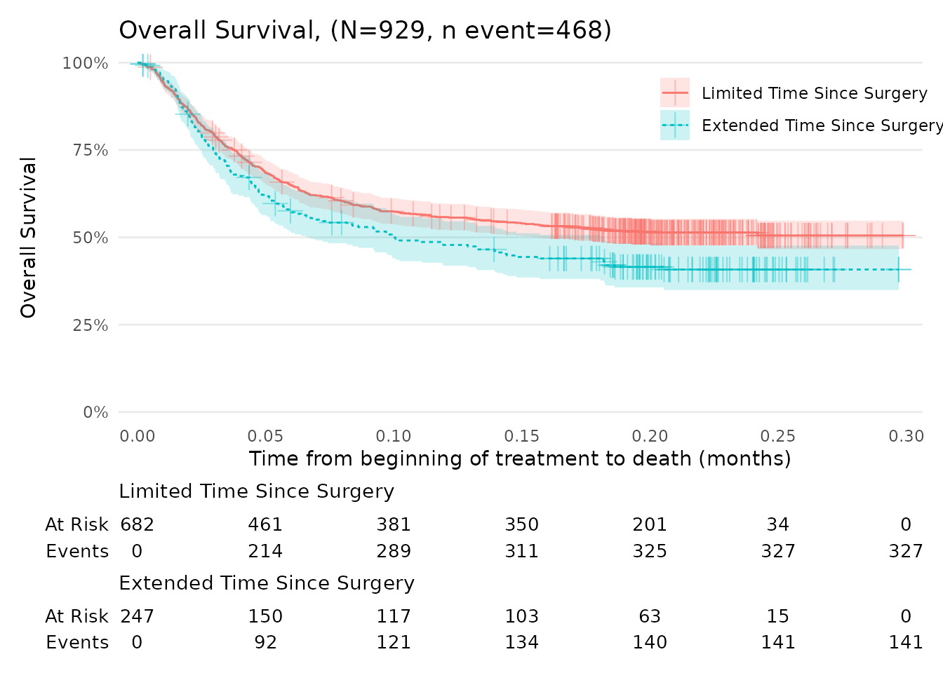
Overall Survival (OS)

The function scale_ggsurvfit() can be used to automatically adjust the axes limits of Kaplan-Meier plots to better fit the data and improve visualisation. Note: The scale_ggsurvfit() function automatically scales the y-axis in percentage.

km_OS = survfit2(Surv(time_OS, status_OS) ~ surg, data = data_surv_v2) %>%
  ggsurvfit(linetype_aes = TRUE) +
  add_confidence_interval() +
  add_risktable(
    risktable_stats = c("n.risk", "cum.event" )
  ) +
  theme_ggsurvfit_KMunicate() +
  scale_ggsurvfit()+
  theme(legend.position = "inside", legend.position.inside = c(0.85, 0.85))

N_total <- nrow(data_surv_v2)
n_event <- sum(data_surv_v2$status_OS == 1)
title_text <- glue("Overall Survival, (N={N_total}, n event={n_event})")


km_OS +
  add_censor_mark(size = 4, alpha = 0.4) +
  labs(
    x = "Time from beginning of treatment to death (months)",
    y = "Overall Survival",
    title =title_text 
  )

Livia Pierotti

2024-11-26

Introduction

Data Overview

Data Preparation

Variable Creation

Kaplan-Meier Analysis

Generate survival estimates using `survfit2()`

Generate survival curves

Progression-Free Survival (PFS)

Overall Survival (OS)

Kaplan-Meier Guideline Suggestions

Livia Pierotti

2024-11-26

Introduction

Data Overview

Data Preparation

Variable Creation

Kaplan-Meier Analysis

Generate survival estimates using survfit2()

Generate survival curves

Progression-Free Survival (PFS)

Overall Survival (OS)

Generate survival estimates using `survfit2()`